Vision Transformers
Bridging the gap between Computer Vision and NLP

Preface
Introduced in the paper, An Image is Worth 16x16 Words: Transformers for Image Recognition at Scale, Vision Transformers (ViT) are the new talk-of-the-town for SOTA image classification. Experts feel this is only the tip of the iceberg when it comes to Transformer architectures replacing their counterparts for up/downstream tasks.

Here, I break down inner workings of Vision Transformer.
Transformer Encoders and Self-Attention
Note: You can skip this part if you’re familiar with Transformers.
Before we get into the ViT architecture, let’s look at Self-Attention and its application in the Transformer Encoder.
Self-Attention is a popular mechanism re-introduced in the paper, Attention Is All You Need. It enables sequence learners to better understand the relationships between different components of the sequences they’re training on. For a given sequence, when a certain component attends to another, it means they are closely related and have an impact on each other in the context of the whole sequence.
For instance, in the sentence, “The horse walked across the bridge”, “across” will probably attend to “bridge” and “horse” since it establishes the context of the sentence. The “horse” is the entity that’s walking across and the “bridge” is the entity being walked across. Through pre-training, these relationships are learned and enforced.
Let’s diagramatically break down this process of running the Self-Attention mechanism.
For a given sequence, the m incoming word vectors of length n are stacked and multiplied by an initial set of weights Wq, Wk, and Wv, of dimensions nxD – this gives us 3 matrices, queries Q, keys K, and values V, of size mxD.
Here, D is the embedding dimension used throughout the Transformer.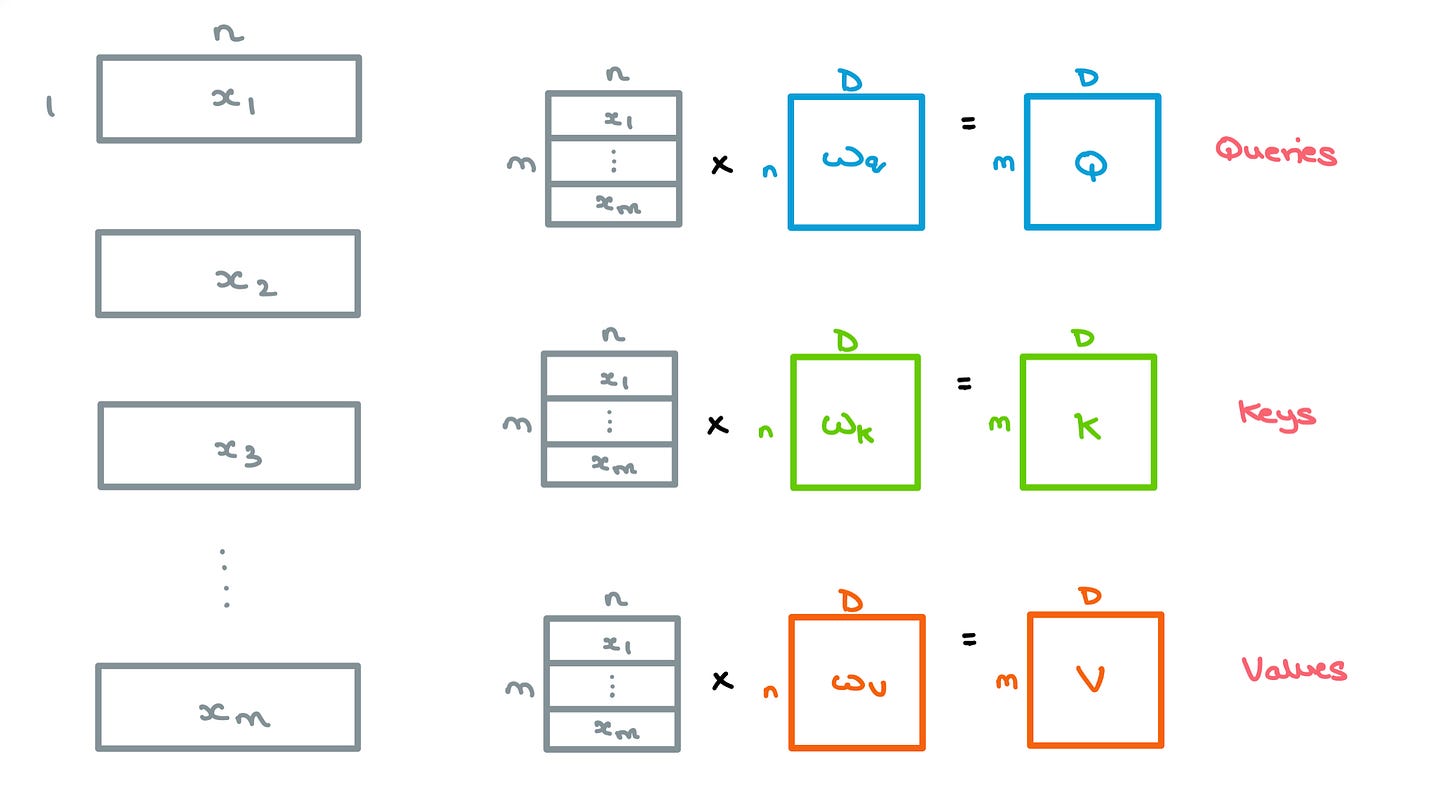
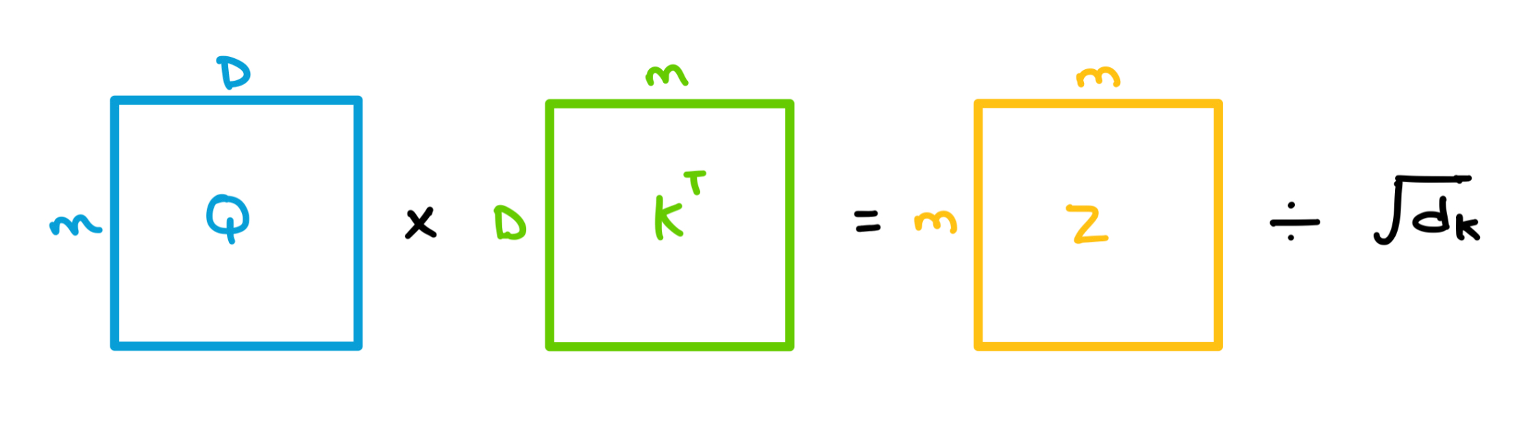
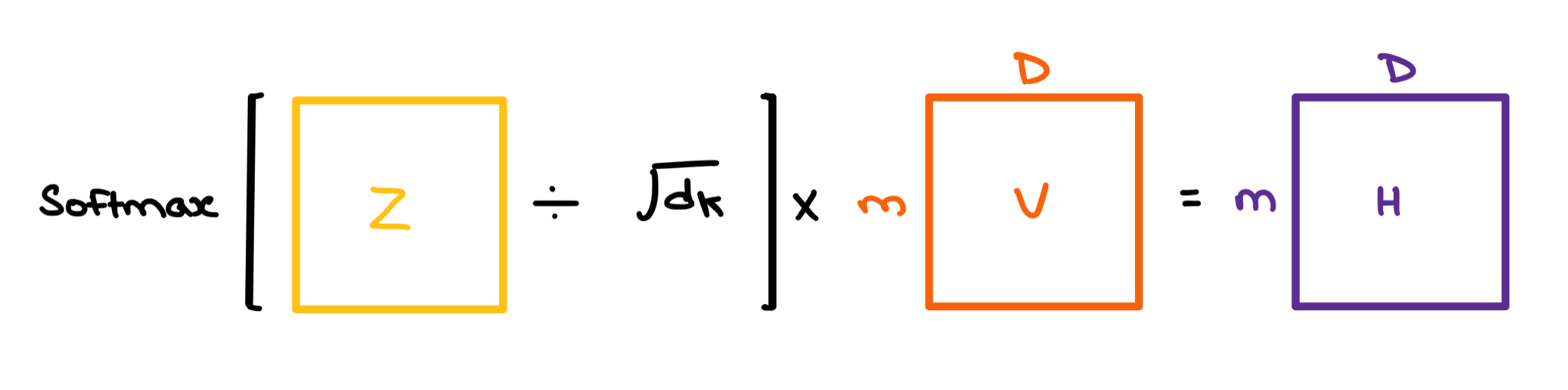
A dot product is taken between each q vector in Q and all the k vectors in K collectively – Linear Algebraically, this means we multiply Q and the transpose of K. This gives us a mxm matrix which we divide by the square root of the dimension of K (
64in the paper) to give us the Attention Matrix Z.This is called Scaled Dot-Product Attention and it’s used to prevent exploding/vanishing gradients.
Without scaling, the dot products grow in magnitude, pushing the Softmax values to regions where gradients are really small during Backpropagation.

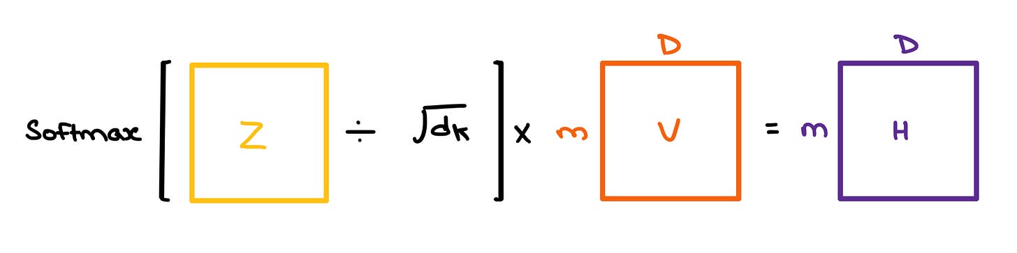
The Softmax of this mxm matrix Z is taken to give us the Attention Weights; it tells us which component vector in the sequence attends to the others. This resulting matrix is multiplied with V to give us the final Self-Attention outputs.

The “Self” in Self-Attention comes from the fact that we’re comparing the component vectors in a sequence with every other vector in said sequence. If a sentence has 5 words, the resulting Attention Matrix will have 5x5 entries depicting the relationships between each word and the others.
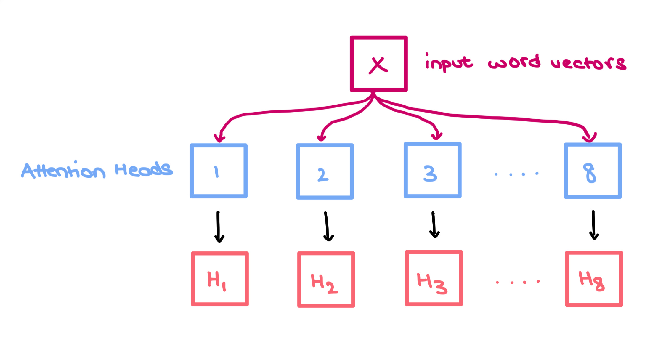
Multi-headed Self-Attention
You can think of each head as an independent “box” performing the 3 sets of operations mentioned above. Each box comes with its own set of independent weights Wq, Wk, and Wv but takes in the same stacked input sequences X.
We do this to increase the predictive power of the Transformer since each head has its own internal representation of the inputs; it allows for a more complete understanding of the relationships between words in a sequence ie. collective, shared knowledge.
We then simply concatenate them to form a larger mxDx8 matrix which we multiply with another set of weights Wo of size 8xDxJ to give us back a mxJ matrix.
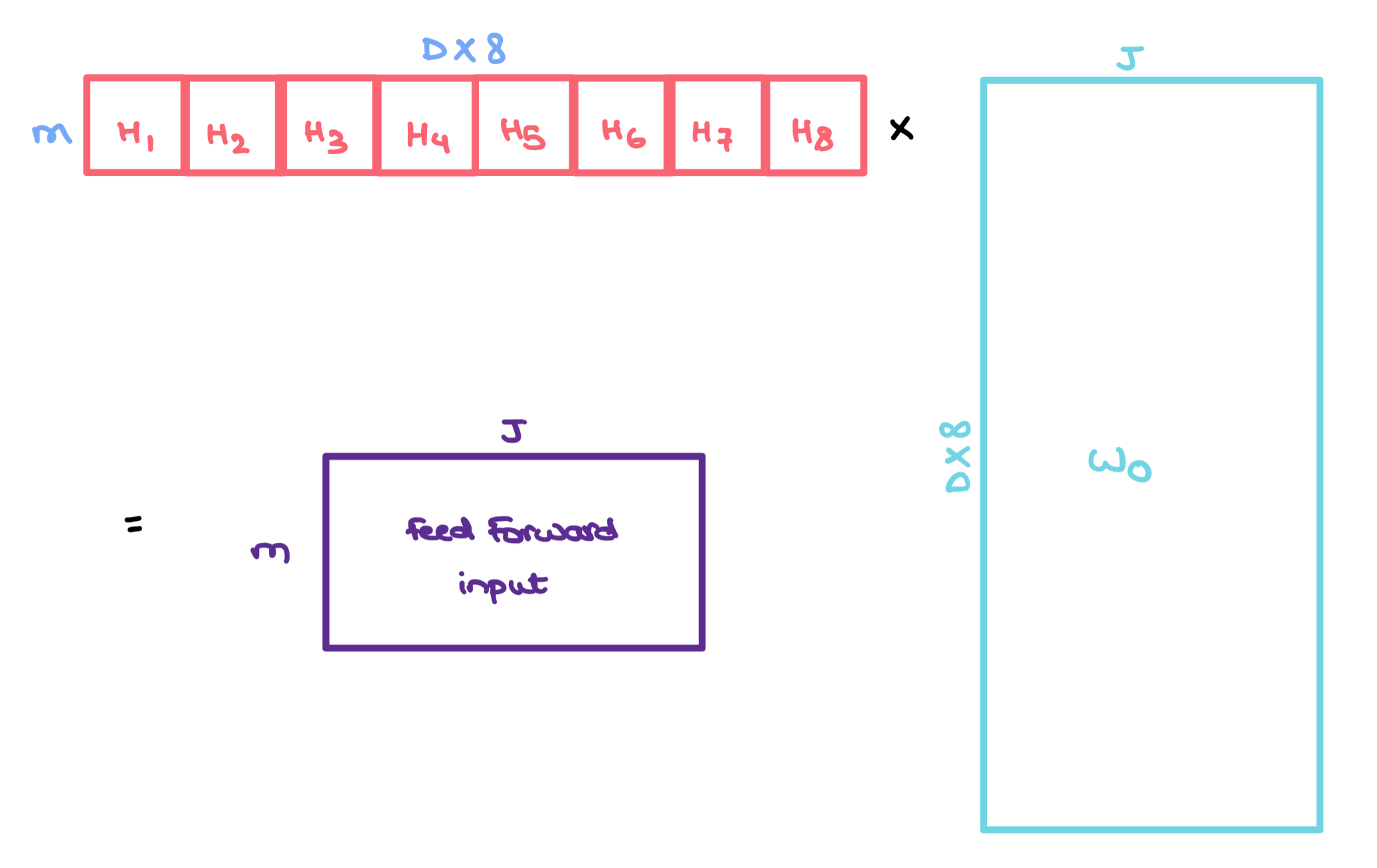
This result matrix captures the information of all the heads and can be sent to a Feed Forward layer with hidden layer dimension J for further processing.
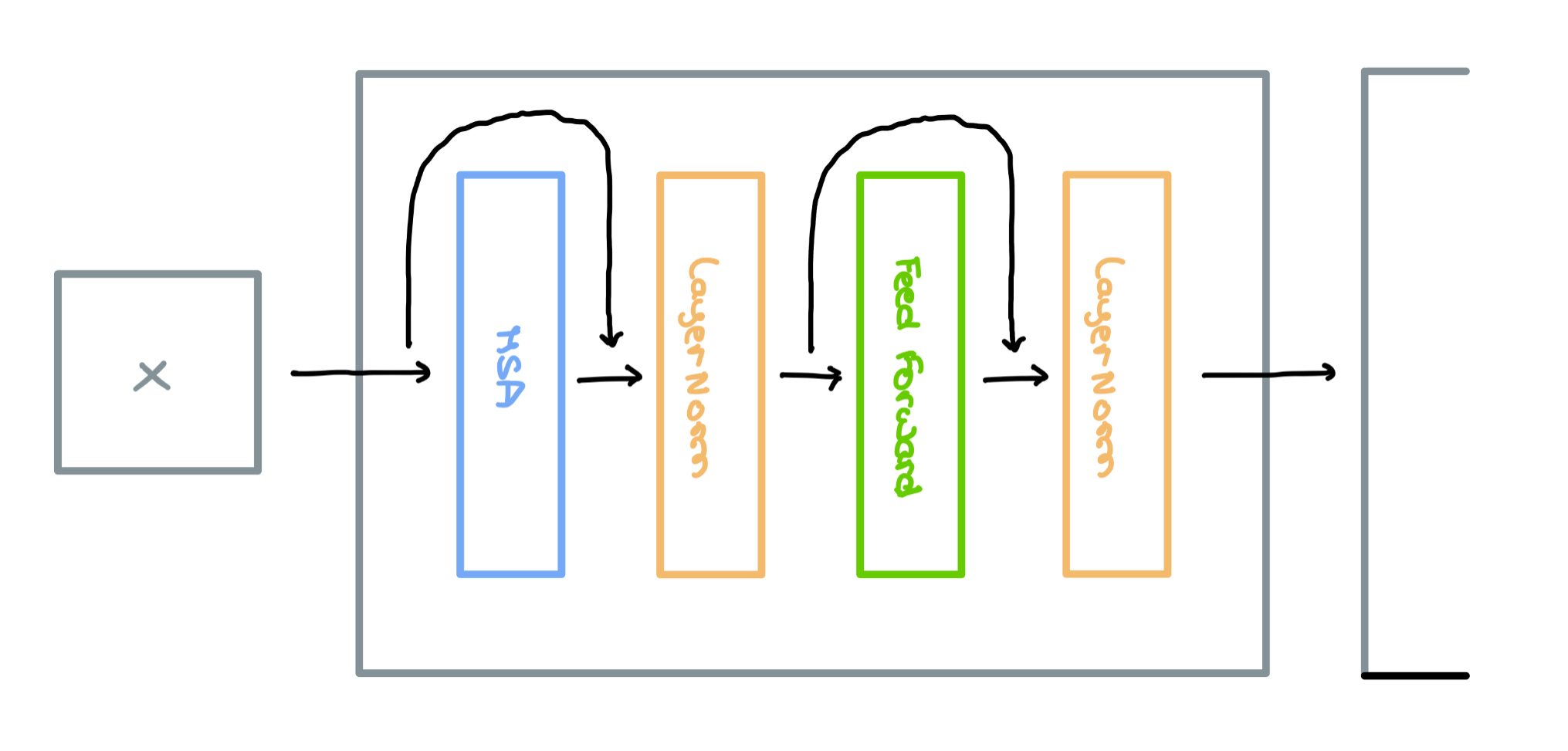
Encoder Block
Multi-headed Self-Attention, LayerNorm, and Feed Forward layers are used to form a single Encoder Block as shown below. The original paper makes use of Residual Skip Connections that route information between disconnected layers.
To find out more about the benefits of adding Skip Connections, check out this article.
Encoder
These Encoder Blocks are stacked one on top of each other to form the Encoder architecture; the paper suggests stacking 6 of these blocks. Sequences are converted into word vectors and sent in for encoding.
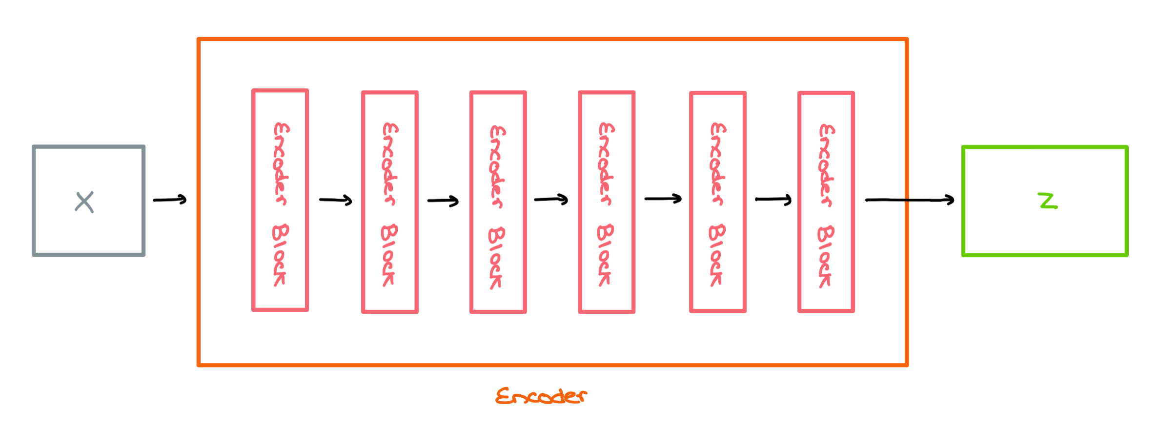
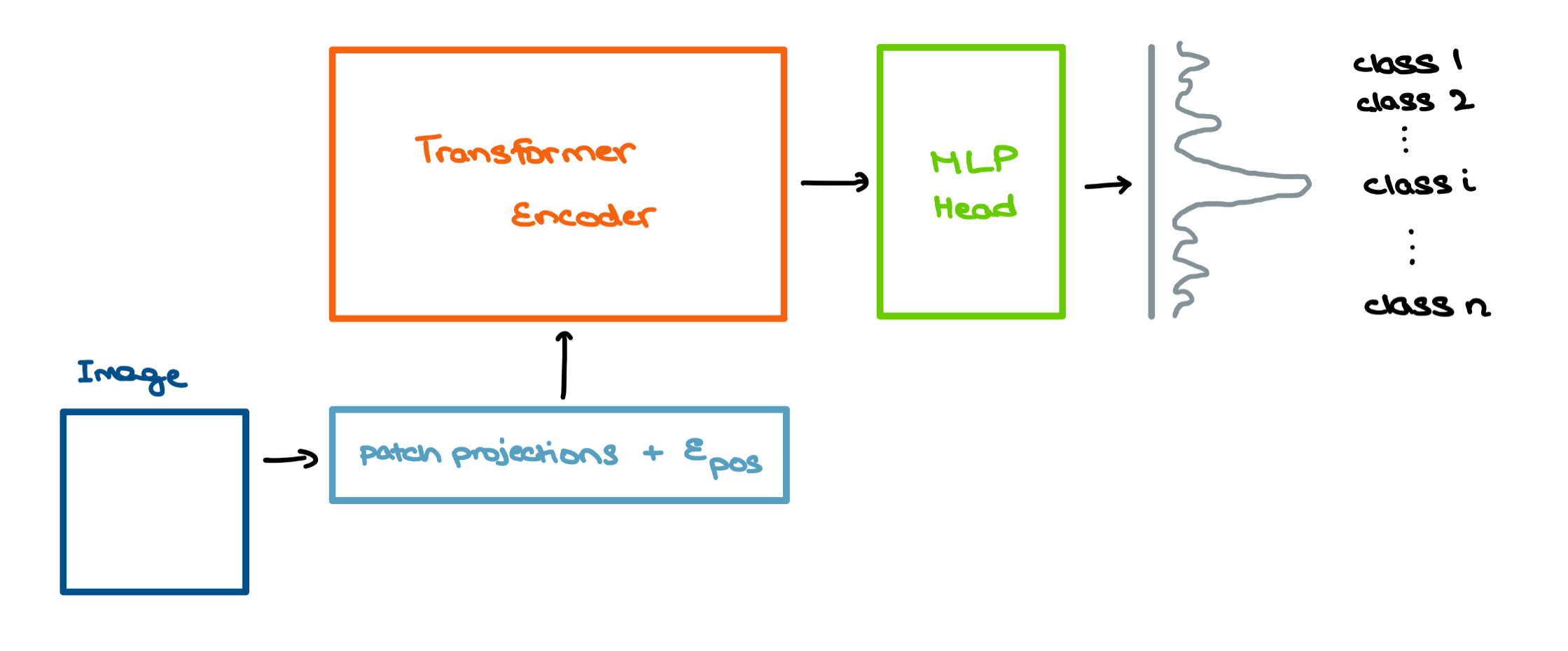
In a regular Transformer, the output Z of the Encoder is sent into the Decoder (not covered). However, in the ViT, it’s sent into a Multilayer Perceptron for classification.
For a complete breakdown of Transformers with code, check out Jay Alammar’s Illustrated Transformer.
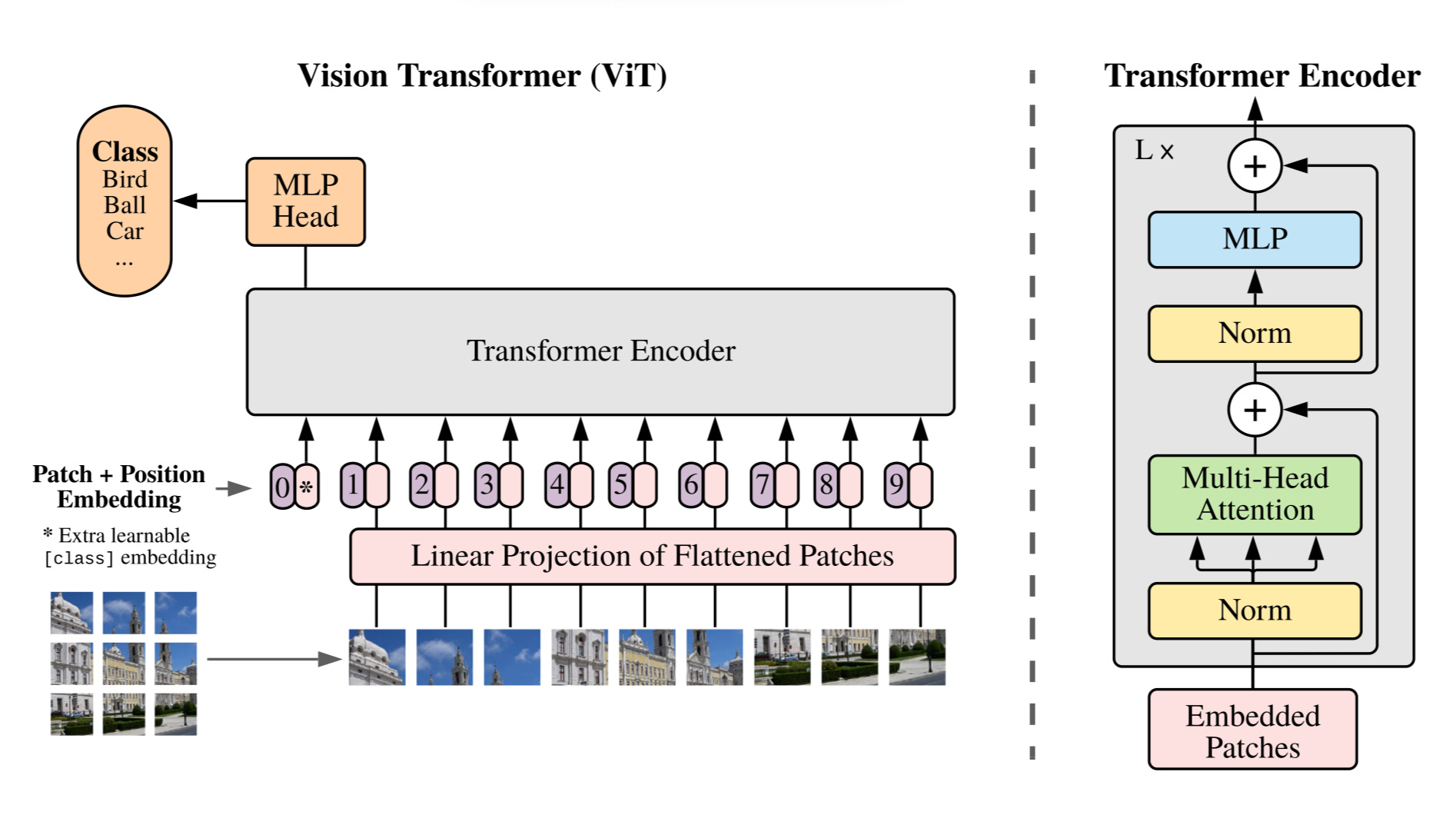
Vision Transformer
Now that you have a rough idea of how Multi-headed Self-Attention and Transformers work, let’s move on to the ViT. The paper suggests using a Transformer Encoder as a base model to extract features from the image and passing these “processed” features into a Multilayer Perceptron (MLP) head model for classification.
Processing Images
Transformers are already very compute-heavy – they’re infamous for their quadratic complexity when computing the Attention matrix. This worsens as the sequence length increases.
For the sake of simplicity, I’m assuming we’re working with a grayscale image with only one colour channel.
The same principle works with multiple channels (like RGB) – only thing changing is the patch dimensions from PxP to PxPxC, where C is the number of channels.
For a standard 28x28 MNIST image from, we’d have to deal with 784 pixels. If we were to pass this flattened vector of length 784 through the Attention mechanism, we’d then obtain a 784x784 Attention Matrix to see which pixels attend to one another. This is very costly even for modern-day hardware.
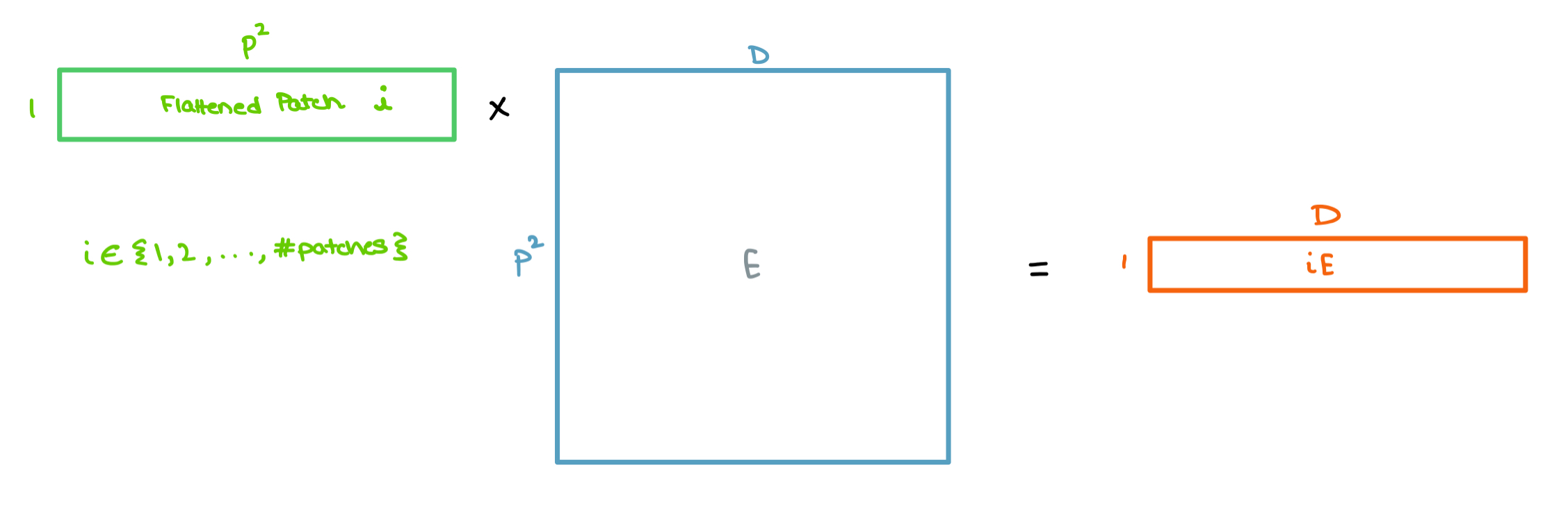
This is why, the paper sugests breaking the image down into square patches as a form of lightweight “windowed” Attention.
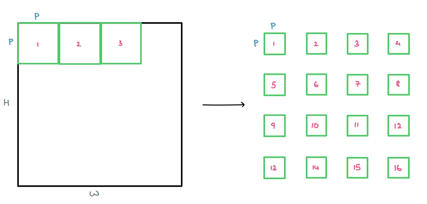
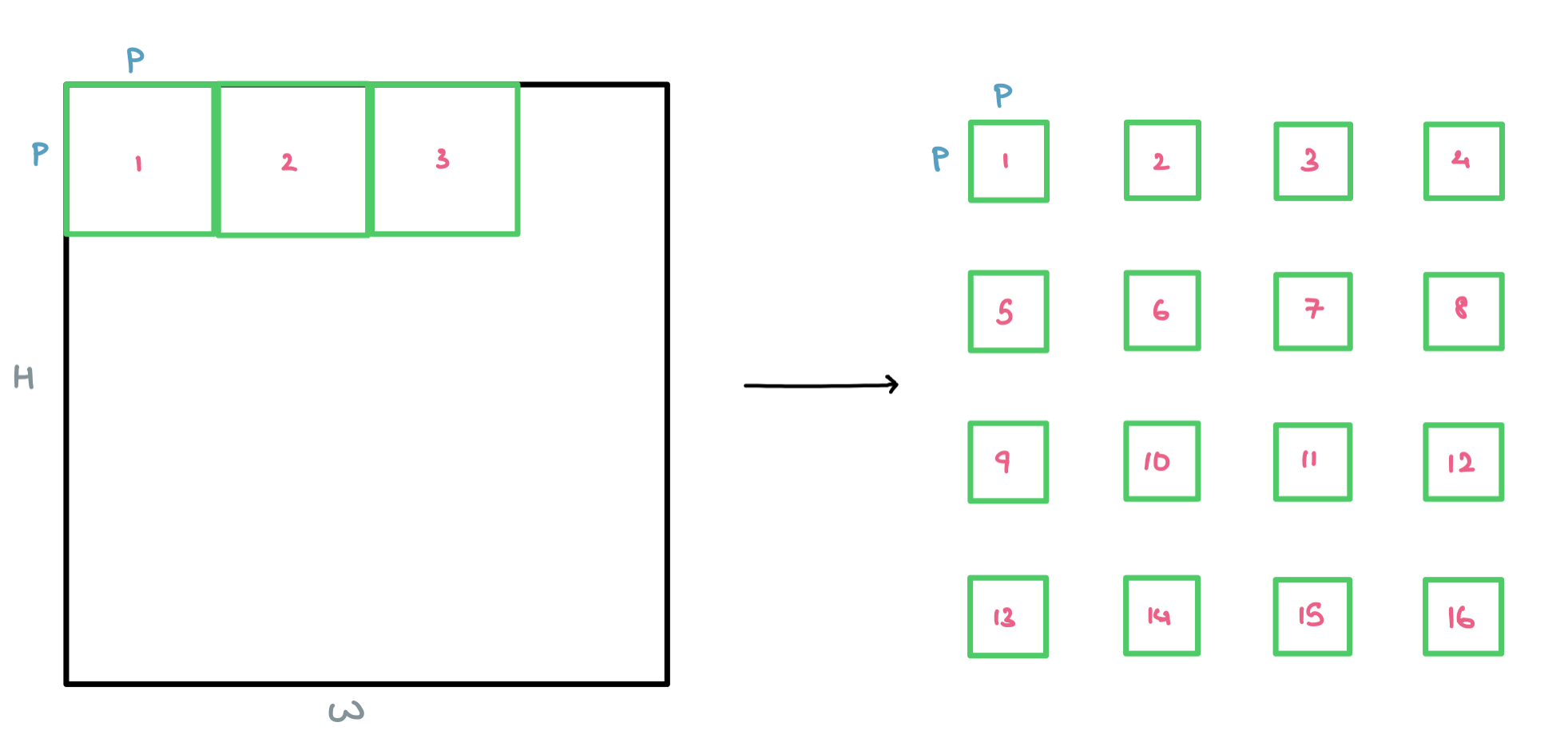
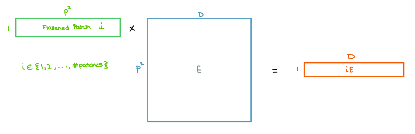
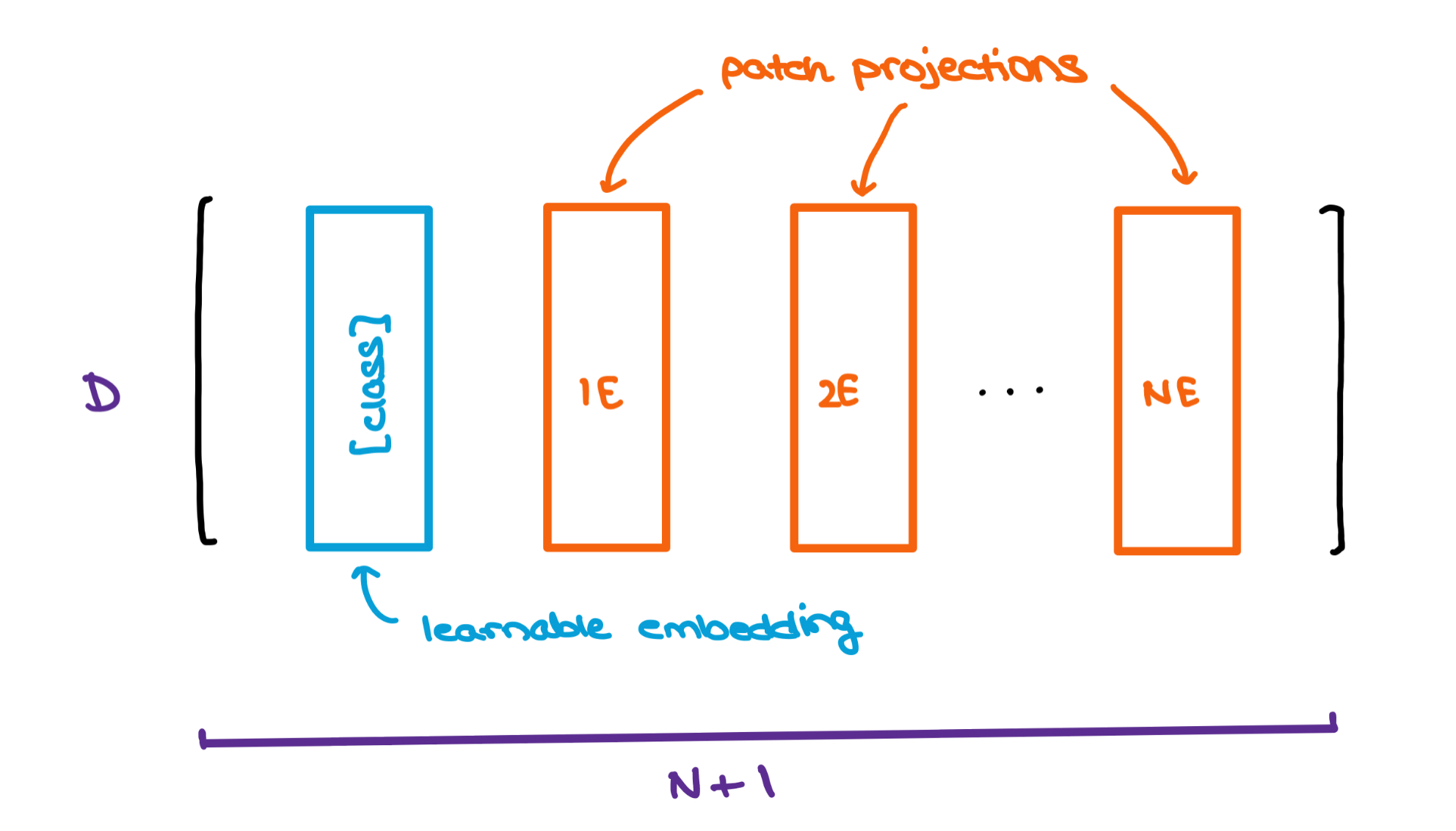
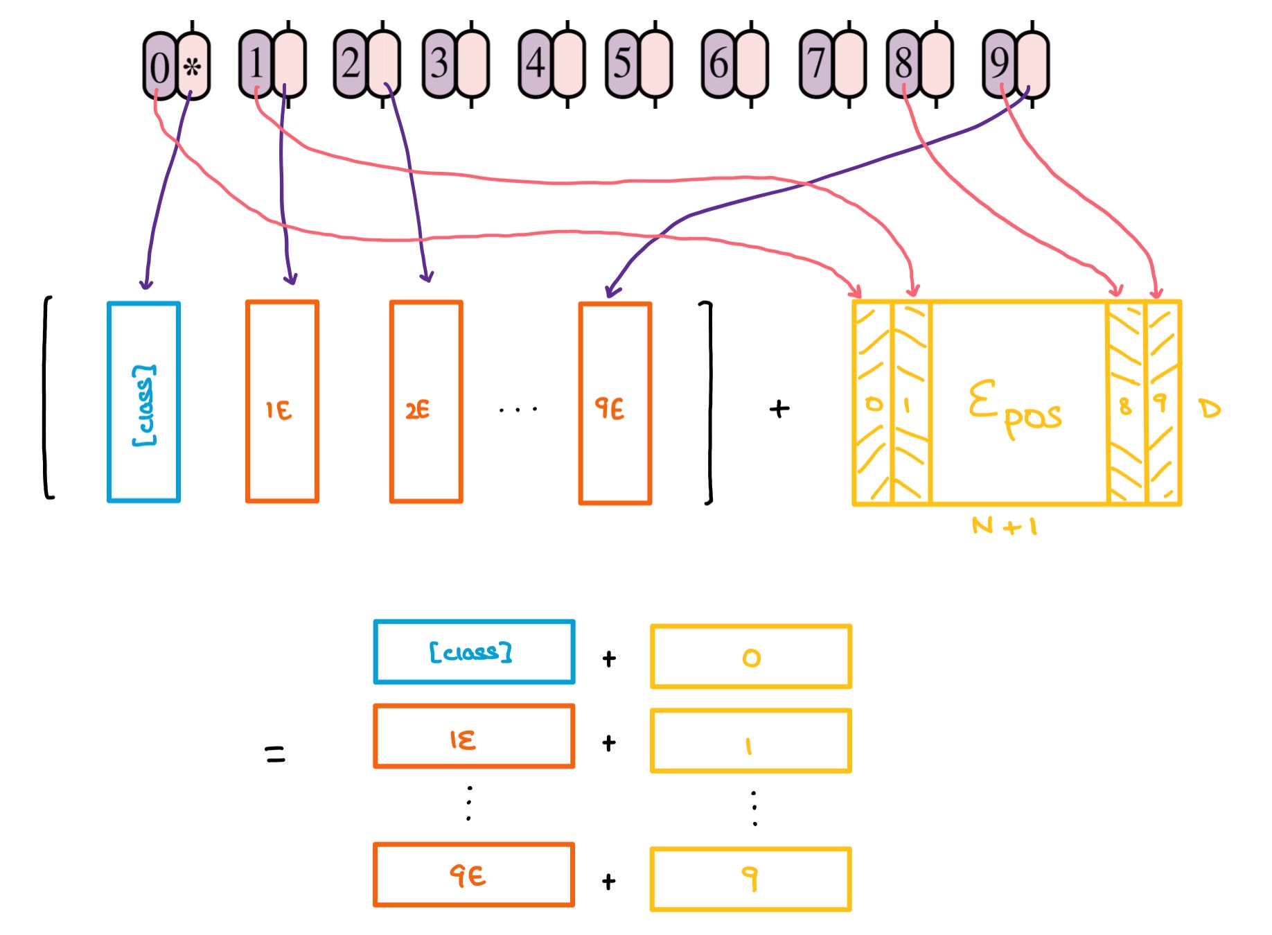
These patches are then flattened and sent through a single Feed Forward layer to get a linear patch projection. This Feed Forward layer contains the embedding matrix E as mentioned in the paper. This matrix E is randomly generated.
To help with the classification bit, the authors took inspiration from the original BERT paper by concatenating a learnable
[class]embedding with the other patch projections. This learnable embedding will be important at a later stage which we’ll get to soon.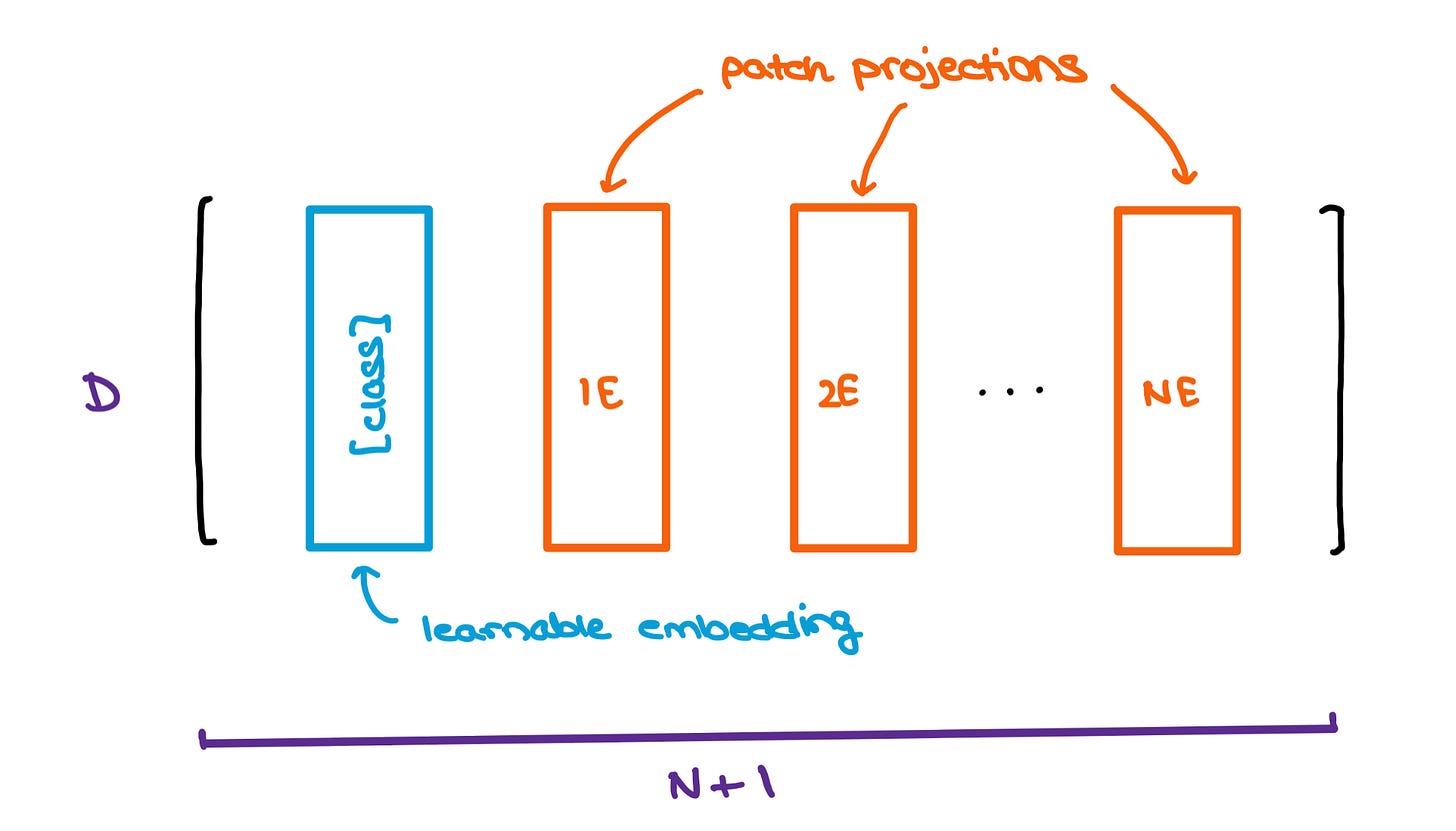
N is the number of patches form the image. Yet another problem with Transformers is that the order of a sequence is not enforced naturally since data is passed in at a shot instead of timestep-wise, as is done in RNNs and LSTMs. To combat this, the original Transformer paper suggests using Positional Encodings/Embeddings that establish a certain order in the inputs.
The positional embedding matrix E_pos is also randomly generated and added to the concatenated matrix containing the learnable class embedding and patch projections.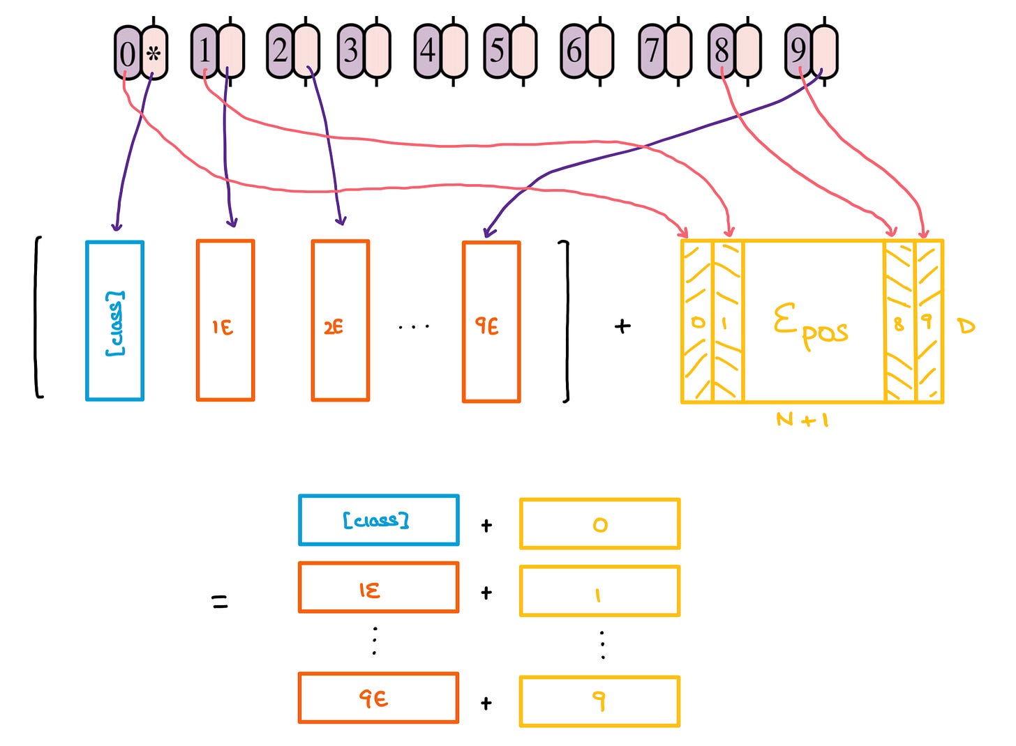
D is the fixed latent vector size used throughout the Transformer. It’s what we squash the input vectors to before passing them into the Encoder. Altogether, these patch projections and positional embeddings form a larger matrix that’ll soon be put through the Transformer Encoder.
MLP Head
The outputs of the Transformer Encoder are then sent into a Multilayer Perceptron for image classification. The input features capture the essense of the image very well, hence making the MLP head’s classification task far simpler.
The Transformer gives out multiple outputs. Only the one related to the special [class] embedding is fed into the classification head; the other outputs are ignored. The MLP, as expected, outputs a probability distribution of the classes the image could belong to.
[class] embedding and ignores the other outputs.In a nutshell
The Vision Transformer paper was among my favourite submissions to ICLR 2021. It was a fairly simple model that came with promise.
It achieved some SOTA benchmarks on trending image classification datasets like Oxford-IIIT Pets, Oxford Flowers, and Google Brain’s proprietary JFT-300M after pre-training on ILSVRC’s ImageNet and its superset ImageNet-21M.
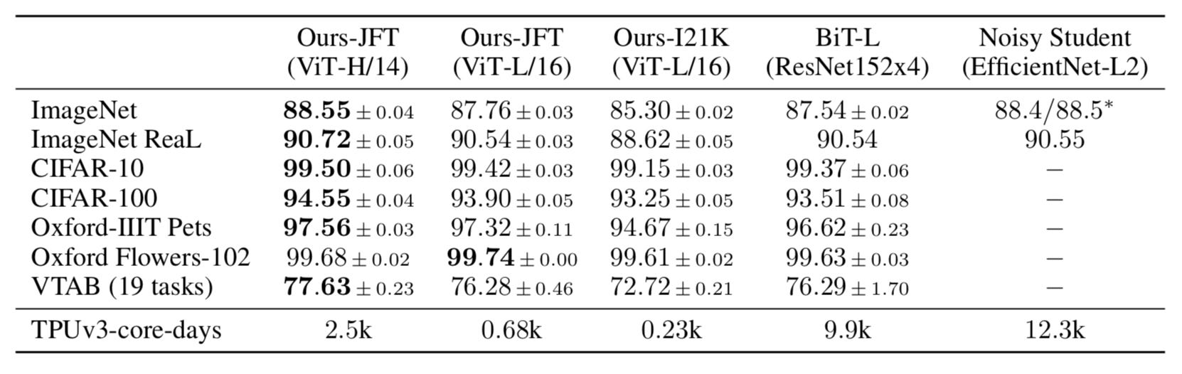
In the Visual Task Adaptation Benchmark (VTAB), it achieves some decent scores in different (challenging) categories.
Transformers aren’t mainstream yet
Sure, these scores are great. Though, I, like many others, still believe we’re far from a reality where Transformers perform most up/downstream tasks. Their operations are compute-heavy, training takes ages on decent hardware, and the final trained model is too large to host on hacky servers (for projects, at least) without severe latency issues during inference. It has its shortcomings that have to be dealt with before becoming the convention in industry (applications.
Yet, this is just the beginning; I’m sure there’ll be tons of research in this area to make Transformer architectures more efficient and lightweight. Till then, we’ve got to keep swimming.
Thanks for reading! I’ll catch you in the next one.
Thanks for sharing!