8-Core Training on Colab TPUs 🏎
Making the most of your TPUs using PyTorch XLA ...

Preface

I recently tweeted this and somehow it popped off (Jeff Dean retweeted it 🥵):
A lot of people asked me how I went about this process. A few had complaints about running into a ton of errors that had no apparent fix. On an unrelated note, it turns out that people prefer Google Colab to run their code based on this very truthworthy poll here.
The process of using Cloud TPUs via jax is a breeze for Googlers. Here’s my conversation thread with a few of them on how they go about doing so. I wish it were that simple for us non-Googlers. Sadly, jax has its associated set of mental gymnastics I do not want to get into.
So, here’s an article that simplifies how to train PyTorch XLA models on all 8 cores of a Colab TPU. The process is rather tedious with many moving parts but you’ll be maximising the compute resources you have at your disposal. Not using all available cores on a Colab TPU is like having to choose between a knife and toothpick to cut a watermelon, but going with the toothpick.
Let’s get started!
If you like what you read, do consider subscribing to my Substack here!
Training on Colab TPUs
1. Changing Runtime
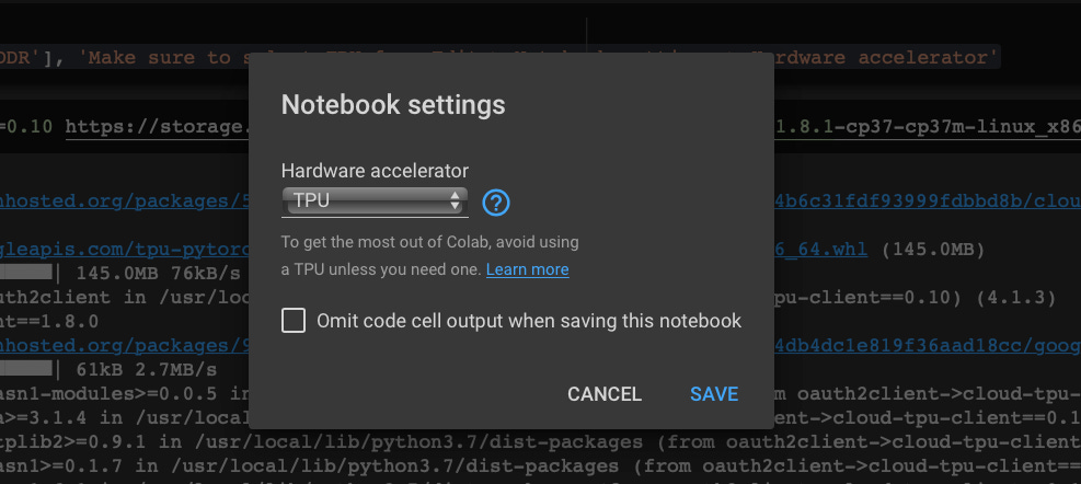
First, you need to enable the TPU runtime. Go to the menu bar and do the following:
Edit > Notebook settings > Hardware accelerator > Click SAVE
Next, check if the TPU configuration has been acknowledged. This shouldn’t print anything if you’ve changed to the TPU runtime.
| import os | |
| assert os.environ['COLAB_TPU_ADDR'], 'Make sure to select TPU from Edit > Notebook settings > Hardware accelerator' |
2. Installations
You’ll need to install PyTorch XLA on the Colab instance. You’ll also need to install a bunch of other libraries that help us with multi-processing.
| # download and install PyTorch XLA | |
| !pip install cloud-tpu-client==0.10 https://storage.googleapis.com/tpu-pytorch/wheels/torch_xla-1.8.1-cp37-cp37m-linux_x86_64.whl | |
| # basic torch sub-modules (feel free to add on [eg: einops, time, random, etc.]) | |
| import numpy as np | |
| import torch | |
| import torch.nn as nn | |
| import torch.nn.functional as F | |
| import torch.optim as optim | |
| # TPU-specific libraries (must-haves) | |
| import torch_xla | |
| import torch_xla.core.xla_model as xm | |
| import torch_xla.debug.metrics as met | |
| import torch_xla.distributed.parallel_loader as pl | |
| import torch_xla.distributed.xla_multiprocessing as xmp | |
| import torch_xla.utils.utils as xu |
These torch_xla modules will help us distribute data and snychronise training across all TPU cores. It’s important to ensure these libraries are imported without any issues.
3. Model Helper Templates
You can create model classes as you normally would with Torch.
| class MyCustomNet(nn.Module): | |
| def __init__(self, myparams): | |
| super().__init__() | |
| # define layers | |
| ... | |
| def forward(self, x): | |
| ''' | |
| Pass your inputs through your layers as you normally would. | |
| No change here. | |
| ''' | |
| return layers(x) |
Warning: Ensure you do not have any alternate devices used within your model class code, be it in
forwardor elsewhere. Basically, do not use.to(device)prematurely; it was my leading cause of failure.You will get the chance to seat your model atop the TPU device soon.
Mapping Operations Across Cores
Here’s where we see some change from the usual way of writing an end-to-end PyTorch pipeline. You’d expect us to preprocess the dataset here. However, PyTorch XLA expects us to create a “map” function that is performed and executed by all workers / cores simultaneously.
Note: I use “core”, “worker”, processor”, and “node” interchangeably. I mean the same thing.
4. Map Function
All our dataset preprocessing, model instantantiation, training, validation, and testing happens inside this map function.
It gets really messy here as we’re about to stuff what usually goes into many code cells into one large code cell containing this map function.
Start off by creating a map function:
| def map_fn(index, flags): | |
| ''' | |
| Contains the following: | |
| - data preprocessing | |
| - model instantiation | |
| - training loop | |
| - validation (optional) | |
| - testing | |
| NOTE: all code beyond this belong inside this unless otherwise stated | |
| ''' |
Here, index is the identifier of the workers. If we use all 8 cores, they’d cover 0 to 7. flags contains some information we will pass in later like number of epochs, batch size, and other hyper-parameters (more on this later).
Beyond this part, all code blocks are inside this
map_fnfunction (i.e., indented inwards once)
5. Dataset Preprocessing
I mentioned that the abovementioned map function is performed by all cores / workers simultaneously. However, we don’t want our dataset to be replicated repeatedly across all cores. For very large datasets, it’d cause memory leaks.
So, we want to instruct the master nodes and worker nodes to download the data only once. To do so, we use the xm.rendezvous(…) function.
| # add your custom transforms and augmentations | |
| T = transforms.Compose([ | |
| transforms.ToTensor(), | |
| ... | |
| ]) | |
| # instructing the master node to download the dataset only ONCE | |
| if not xm.is_master_ordinal(): | |
| xm.rendezvous('download_only_once') | |
| mnist_train = datasets.MNIST(..., train=True, transform=T, download=True) | |
| mnist_test = datasets.MNIST(..., train=False, transform=T, download=True) | |
| if xm.is_master_ordinal(): | |
| xm.rendezvous('download_only_once') |
Next, we can go about creating our data generators for training and testing. We also have to create a sampler that’s multi-processing-friendly. For that, we can use the DistributedSampler object.
| ''' | |
| num_replicas is the total number of times we'll replicate | |
| the batch samples for all cores. | |
| ''' | |
| train_sampler = torch.utils.data.distributed.DistributedSampler( | |
| im_train, | |
| num_replicas=xm.xrt_world_size(), | |
| rank=xm.get_ordinal(), | |
| shuffle=True | |
| ) | |
| test_sampler = torch.utils.data.distributed.DistributedSampler( | |
| im_test, | |
| num_replicas=xm.xrt_world_size(), | |
| rank=xm.get_ordinal(), | |
| shuffle=False | |
| ) | |
| # ignore batch_size and num_workers for now | |
| train_loader = torch.utils.data.DataLoader( | |
| im_train, | |
| batch_size=flags['batch_size'], | |
| sampler=train_sampler, | |
| num_workers=flags['num_workers'], | |
| drop_last=True | |
| ) | |
| test_loader = torch.utils.data.DataLoader( | |
| im_test, | |
| batch_size=flags['batch_size'], | |
| sampler=test_sampler, | |
| num_workers=flags['num_workers'], | |
| drop_last=True | |
| ) |
You can ignore flags[‘batch_size’] and flags[‘num_workers’] for now. I’ll get to that soon when we cover flags. Here, the xm.xrt_world_size() gives us the total number of cores we’ll be training on. If we use all 8 cores, this number would be 8 (or whatever is available). xm.get_ordinal() gets the index of the core in context (it’s like the index variable we pass into the map function).
Loading Data from Local Colab Directory
I know some of you download your datasets from the internet and load them in using datasets.ImageFolder(…). You can do that here too! Though, take note of these instructions very very carefully:
You will have to download the dataset using wget (and untar/unzip if you have to) outside the cell containing map_fn.
| !wget http://www.some_dataset_website.com/my_dataset.tar.gz | |
| !tar -xvzf my_dataset.tar.gz |
Only after doing this in the cell above, you can replace the original code in map_fn with this directory loading code:
| PATH = "./my_dataset/" # path to dataset on Colab instance | |
| TRAIN_PATH = PATH + "train/" | |
| VAL_PATH = PATH + "val/" | |
| # your custom augmentations | |
| T = transforms.Compose([ | |
| transforms.ToTensor(), | |
| ... | |
| ]) | |
| # same procedure but you use datasets.ImageFolder(...) instead | |
| if not xm.is_master_ordinal(): | |
| xm.rendezvous('download_only_once') | |
| data_train = datasets.ImageFolder(TRAIN_PATH, transform=T) | |
| data_test = datasets.ImageFolder(VAL_PATH, transform=T) | |
| if xm.is_master_ordinal(): | |
| xm.rendezvous('download_only_once') |
6. Model Instantiation
This is a fairly simple procedure. Though, you’ll have to seat it atop the right device. Otherwise, you’re in for a major headache.
| device = xm.xla_device() | |
| # define some hyper-params you'd feed into your model | |
| in_channels = ... | |
| random_param = ... | |
| # create model using appropriate hyper-params | |
| net = MyCustomNet(...) | |
| # seat it atop the TPU worker device and switch it to train mode | |
| net = net.to(device).train() | |
| # get the loss function and optimizer – use anything | |
| criterion = nn.CrossEntropyLoss() | |
| optimizer = optim.Adam(net.parameters(), lr=..., betas=(...)) |
So, if we use all 8 cores, we have access to workers 0 through 7. The device variable allows us to access the specific worker node. It’ll be of the form “TPU:i” where i ranges from 0 to 7 (eg: TPU:2, TPU:5).
If you’ve used Colab GPUs before, you’ll recognise the notation style. The CUDA GPU device is identified by “
cuda:0”. It’s the same concept here!
7. Training and Testing Loop
This part of the map function is simple too and doesn’t have too many changes. We train the model for some N epochs across a few batches, get the validation accuracy at the end of each epoch, and finally exit the loop.
Though, one thing to note is that we use a specialised type of data loader meant for multi-processing. We’ll be sending our train_loader and test_loader into a ParallelLoader that handles the cross-worker batch loading. It takes in the specific work and data loaders we created earlier.
| # hlper function to get the testing accuracy at the end of the epoch | |
| def get_test_stats(model, loader): | |
| total_samples = 0 | |
| correct = 0 | |
| model.eval() # switch to eval mode | |
| for (batch_idx, data) in enumerate(loader, 0): | |
| x, y = data | |
| logits = model(x) | |
| preds = torch.argmax(logits, 1) | |
| correct += torch.eq(y, preds).sum().item() | |
| total_samples += flags['batch_size'] # more on flags later | |
| accuracy = 100.0 * (correct / total_samples) | |
| return accuracy | |
| EPOCHS = 10 # feel free to change | |
| for epoch in range(EPOCHS): | |
| # (optional) calculate the batch-wise loss | |
| running_loss = 0 | |
| steps = 0 | |
| model.train() # switch to train mode since we will switch to eval mode later | |
| # get the specialised parallel train loader | |
| para_loader_train = pl.ParallelLoader(train_loader, [device]).per_device_loader(device) | |
| for (batch_idx, data) in enumerate(para_loader_train, 0): | |
| steps += 1 | |
| x, y = data | |
| output = net(x) | |
| loss = criterion(output, y) | |
| optimizer.zero_grad() | |
| loss.backward() | |
| running_loss += loss.item() | |
| xm.optimizer_step(optimizer) | |
| if (i % 20 == 0): # print stuff out to console | |
| xm.master_print('{} | RunningLoss={} | Loss={}'.format( | |
| batch_idx, running_loss / steps, loss.item()), | |
| flush=True | |
| ) | |
| xm.master_print("Finished training epoch {}".format(epoch)) | |
| # get the specialised parallel test loader | |
| para_loader_test = pl.ParallelLoader(test_loader, [device]).per_device_loader(device) | |
| val_accuracy = get_test_stats(model, para_loader_test) | |
| xm.master_print("Validation Accuracy: {}".format(val_accuracy)) |
I want you to observe a few things here:
Notice how we create our parallel train and test loaders to feed data into the model across all cores.
Notice
xm.optimizer_step(…)function. It updates the model’s weights across all cores at a shot.Notice the
xm.master_print(…)function. Since we have 8 cores doing the same thing, if you use Python’sprint, you’d get the same message printed 8 times. To avoid that,master_printprints any string only once.
8. Running the Map Fuction
Finally, we’ve created our map function. It allows all cores to perform the same set of operations but synchronises everything under the hood.
Note: The code shown here is in a new cell outside the map function without any indentation.
In earlier code blocks you may have noticed flags being used to indicate various hyper-parameters like batch size and number of workers. Here’s where we bring them in.
Likewise, xm.spawn(…) asks the Colab instance to spin up 8 processors and perform whatever is inside map_fn. Though, be warned that this spin up step takes a while to run. It took me 7 minutes to train on CIFAR10 (images resized to 224x224) using ResNet50. Not sure what is the deciding factor but please be patient 😅.
| ''' | |
| Configures some pipeline hyper-parameters. You | |
| can set them to whatever you please. | |
| You have the option of either mentioning it here | |
| or creating variables inside the map_fn function. | |
| This is entirely up to you. I do both for demonstration purposes. | |
| ''' | |
| flags = {} | |
| flags['batch_size'] = 32 | |
| flags['num_workers'] = 8 # we want to train on all 8 cores | |
| flags['num_epochs'] = 10 # I already had the EPOCHS variable in map_fn | |
| flags['seed'] = 42 | |
| # start the 8-core TPU and run map_fn on all workers | |
| xmp.spawn(map_fn, args=(flags,), nprocs=8, start_method='fork') |
In a Nutshell
Figuring out how to use Colab TPUs with PyTorch XLA was a fun task! Although there weren’t many resources around, it was both daunting and exciting to piece together what goes where.
Common Errors
Before I end off, here are two very common errors I ran into and what I suspect is the issue based on my quick fixes. They are definitely not the exact message but are pretty similar:
Tensor is of typetorch.FloatTensor, notXLATensor: one or more tensors you are using are on the wrong device (usually CPU and not the TPU worker). You either forgot to use.to(device)on your model or used it prematurely when testing your model’s outputs and internal dimensions.“device:0” not found: You probably used.to(device)prematurely inside a helper function or some tensor used for testing. Ensure that only the model is seated on the device. The other modules like data loaders manage the data side for you.
I hope this article helps you start training on Colab TPUs. They are an amazing resource to have, especially because they are free of cost and have no strings attached.
Warning: One pesky issue is that you have to be around your computer as it’ll bring up the CAPTCHA popup every once in a while. In the case you don’t tick the box in time, it’ll shut down the instance immediately. You’ll have to start all over again.
If you like what you read, do consider subscribing to my Substack here!